Educational / Student Teams

Differential Drive Robot Simulation

Cal Poly ME 322 · Individual Project · Spring 2026

Developed nonlinear and linearized MATLAB/Simulink models of a Romi differential-drive robot to simulate wheel, chassis, and global-position dynamics under independent motor-voltage inputs.

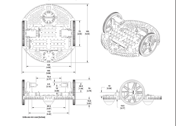
Differential-drive Romi robot simulation — Nonlinear simulation of a Romi differential-drive robot modeled with coupled motor, wheel, and chassis dynamics.

Overview

Developed a nonlinear dynamic model of a Romi differential-drive robot and compared its response against a Jacobian-linearized state-space model across multiple driving conditions.

My Role

Developed the system hand calculations using linear graph theory, derived and augmented the nonlinear state equations, used MATLAB's Symbolic Math Toolbox to linearize the model, implemented both nonlinear and linear simulations in Simulink, and evaluated their response under four voltage-input cases.

Project Overview

This project modeled the dynamic behavior of a two-wheeled Romi robot driven by independent left and right DC gearmotors. The model combined electrical motor dynamics, wheel-ground traction, rigid-body kinematics, and coordinate transformations to predict the robot's motion. A Jacobian-linearized state-space model was developed alongside the full nonlinear model so their responses could be compared across multiple driving conditions.

System Modeling & Hand Calculations

I first developed the transducer relationships, linear graph, normal tree, and nonlinear state equations for the differential-drive system. The hand calculations established how the left and right motors, wheels, and chassis interacted, while the augmented equations added global position and heading states to represent the robot's path.

First page of differential-drive robot hand calculations — Initial system modeling and transducer relationships.

Second page of differential-drive robot hand calculations — Linear graph development for the differential-drive system.

Third page of differential-drive robot hand calculations — Normal-tree development and system relationships.

Fourth page of differential-drive robot hand calculations — Nonlinear state-equation development.

Fifth page of differential-drive robot hand calculations — Augmented kinematic equations for robot heading and position.

Sixth page of differential-drive robot hand calculations — Final state equations used for simulation.

Nonlinear & Linearized Simulation

The nonlinear model was implemented in Simulink using the derived state equations and numerical integration. MATLAB's Symbolic Math Toolbox was then used to determine equilibrium conditions and calculate the Jacobian matrices required for the linear state-space approximation. Both models received identical left- and right-motor voltage inputs, allowing their wheel speeds, chassis motion, and predicted paths to be compared directly.

Simulation Results

Four driving cases were simulated to evaluate straight-line motion, turning, delayed motor actuation, and low-voltage behavior. The results illustrate where the linearized model closely represents the nonlinear system and where the approximation becomes less accurate as the operating condition changes.

Case 1 differential-drive robot velocity comparison — Case 1: Linear and nonlinear response with equal 6 V inputs to both motors.

Case 1 differential-drive robot path comparison — Case 1: Predicted robot path with equal 6 V inputs to both motors.

Case 2 differential-drive robot velocity comparison — Case 2: Linear and nonlinear response with 7 V applied to the left motor and 5 V to the right motor.

Case 2 differential-drive robot path comparison — Case 2: Predicted turning path produced by unequal motor voltages.

Case 3 differential-drive robot velocity comparison — Case 3: Linear and nonlinear response with a delayed 6 V input to the right motor.

Case 3 differential-drive robot path comparison — Case 3: Predicted path produced by delayed actuation of the right motor.

Case 4 differential-drive robot velocity comparison — Case 4: Linear and nonlinear response with equal low-voltage inputs of 1.5 V.

Case 4 differential-drive robot path comparison — Case 4: Predicted robot path under equal low-voltage inputs.

Model Comparison

The simulation results demonstrate the strengths and limitations of linearizing a nonlinear system. The linearized model can closely match the nonlinear response near its operating point, while larger changes in motor input or robot motion can produce increasing disagreement. The animation compares the two simulated robots directly and makes this divergence visible in their predicted paths.